\(\definecolor{frog}{rgb}{1,0,0}\) \(\newcommand{\dx}{\,\text{d}x}\) \(\newcommand{\du}{\,\text{d}u}\) \(\newcommand{\dy}{\,\text{d}y}\) \(\newcommand{\dt}{\,\text{d}t}\)

2 Week 2 – Code demonstrations

Some equations, again. Notice this chapter includes the following code (in _metadata.yml):

---
filters:
    - acc-tools
---

This loads the bonus accessibility features extension. There is a global code toggle button bottom left, and the R and P keyboard buttons will switch all code tabs simultaneously to the chosen language.

Documentation for it can be found here: UofGStats/acc-tools repo

If you plan to use it in all (or most) chapters, then you can just turn it on globally by instead putting this filters code above to the _quarto.yml file. Then disable features on a chapter-by-chapter basis.

\[\frac{\!\textrm{d}^{3} y}{\textrm{d}x^{3}}\]

\[\int_0^{\infty} x^2 \dx \tag{2.1}\]

This equation was called Equation 2.1.

2.1 Features

• You’ll first note in the bottom left is a global toggle button set. You can change all code blocks to R or to Python, by clicking; or by pressing R or P on the keyboard.

2.2 New Section Title

Hidden here is a setup block of R code to load packages and set graph sizes.

```{r}
#| label: reticulate-setup
library(reticulate)
#These next two lines need to run ONCE on your machine
#reticulate::virtualenv_create("r-quarto")
#reticulate::py_install(c("pandas","seaborn","matplotlib","numpy"), envname = "r-quarto")
reticulate::use_virtualenv("r-quarto", required = TRUE)
```

Another standard callout box.

TipBeetle mortality

Jump to the Beetle code.

This is an R .panel-tabset environment. It’s the recommended route to display more than one codeblock at once, switchable via a tab on the top edge.

To make life easier, my extension also adds a global-toggle button which can be used by clicking (see bottom left), or just pressing R or P to toggle all code blocks to R or Python respectively. I’ve also tidied up their appearance, made the tabs more prominent and easier to navigatve with a keyboard.

The code blocks themselves are just like usual RMarkdown blocks you define a language and decide if you want the code to be shown, and if you want the results to be rendered on the screen too.

R

The code in the R example is folded by default. Click on Code to reveal it.

beetles <- read.csv(url("http://www.stats.gla.ac.uk/~tereza/rp/beetles.csv"))
beetles

    dose number killed
1 1.6907     59      6
2 1.7242     60     13
3 1.7552     62     18
4 1.7842     56     28
5 1.8113     63     52
6 1.8369     59     53
7 1.8610     62     61
8 1.8839     60     60

Python

import pandas as pd
beetles = pd.read_csv("../resources/data/beetles.csv")
beetles

2.3 Figures

Quarto calls various different things Figures. See Quarto figures.

In particular, including external images (pre-generated) can be done in many ways and are regarded as figures. However, so are plots generated by R, and indeed any computational blocks of code you want it to run in R or Python.

As usual you use ```{r} to start an R block (which you want to run), and ```{python} for python.

To include pre-rendered images the typical format is inline like this:

![Elephant](elephant.png){fig-alt="A drawing of an elephant."}

The word Elephant from the first bracket becomes the caption and the fig-alt determines the alt-text for screenreaders. A lot more options for controlling size and layout are in the Quarto documentation.

TipInformation on accessibility

For accessibility purposes there a number of actions you should always be taking, but may not be used to.

1. Always add an alt-text to your images. These are designed to be read aloud and describe what someone looking at the image is suppose to get from it. There is lots of advice online for what good alt-text looks like. It’s a particularly rich topic in maths/stats where a plot may need a moderately long description to provide for a non-sighted user what you wish sighted users to have got from it.

2. Always add alt-text to R or Python generated plots, the recommended approach has changed in recent years, now you use the #| syntax to add properties of your blocks.

Here’s an example:

```{r}
#| label: fig-myplot
#| fig-cap: "Here's my caption"
#| fig-alt: "This is the possibly long alt text describing the plot"
#| code-fold: show

plot(cars)
```

Figure 2.1: Here’s my caption

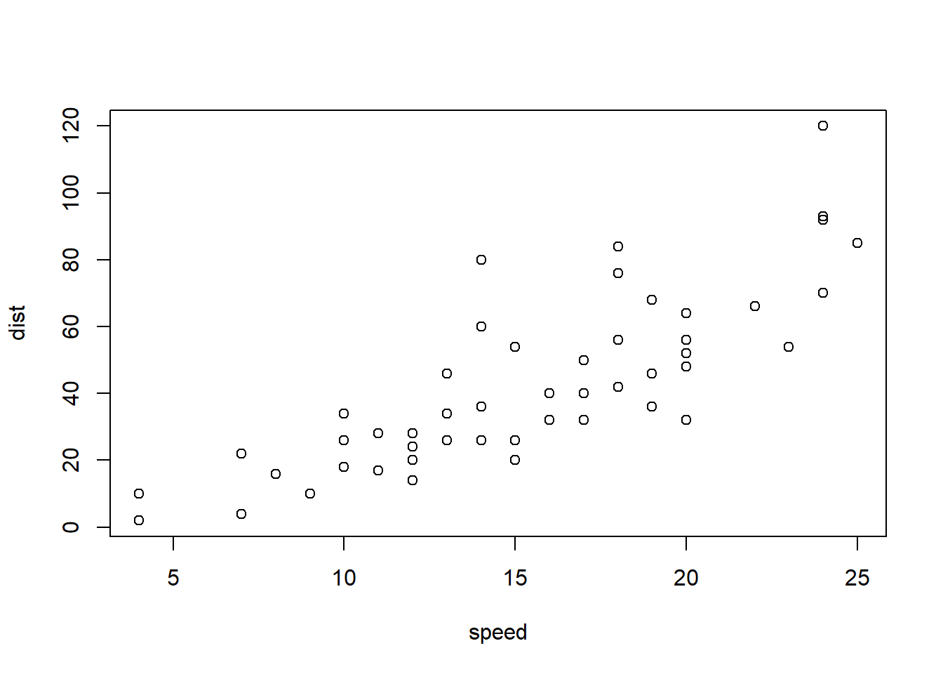
Note that by default the code which generated the plot is also shown. This was made foldable (in the HTML version) with #| code-fold: show but could be hidden entirely with options like #| echo: false.

This figure caption is written in a dark font color. The Quarto default is often too pale and fails accessibility checks, so the acc-style files in my extension fix this, along with a few other things like it (table of contents contrast too).

Python

3+34

R

34+3

[1] 37

Python

5+4

R

4+5

[1] 9

Note that our plot before was called #fig-myplot so we can use @fig-myplot to reference Figure 2.1.