This chapter shows off some nice coloured boxes. They come from the custom-numbered-blocks extension. First you need to install the extension quarto add ute/custom-numbered-blocks.
The following colour definitions need to be added somewhere (e.g. _quarto.yml or _metadata.yml or at the top of this .qmd file) to load the coloured boxes. In this template I have added a link to a file called _numbered-boxes.yml from inside _quarto.yml. In this way you just need to look insider _numbered-boxes.yml to edit the settings.
It looks approximately like this, you define groups of like-numbered boxes, and then define specific classes (and their names later). They can have separate colour schemes too.
We’ve defined several custom-numbered block types using the custom-numbered-blocks option. The key point is that these can be numbered and follow grouped numbering conventions.
Each block belongs to a group that determines its shared numbering.
All of these blocks are foldable, meaning they can be opened and closed. The collapse setting determines the starting state. Most boxes have been set to be open (collapse: false) at the group level, but this can be overridden at both lower levels. e.g. Corollary shares numbering with all the theorem-like boxes, which are all open by default. Corollaries could be all set to closed by default, or even on a case by case basis in the code.
Table 4.1: This is the table’s caption
Box Name
Group
Title Background Color
Left Border Color
Default State
Theorem
thmlike
#948bde
#584eab
Open / Closeable
Lemma
thmlike
#b2dac4
#004721
Open / Closeable
Corollary
thmlike
#7fbad7
#005398
Open / Closeable
Definition
deflike
#ffdc36
#ffb948
Open / Closeable
Video
videolike
#d18888
#660000
Closed / Openable
These boxes also have dark-mode versions, see below. Notice this table had a caption, and it can be referenced with normal Quarto syntax: Table 4.1. They can also have styling added.
Note: The two colors defined for each group represent the left border and the title background.
Here’s an alternative to treating videos as float/figures, just stick them directly onto the page immediately (not as a floating object) but wrap them in a coloured box and use the title of the box to describe the video.
Video 1: Binomial response models applied to beetle mortality data (9m59)
There is some text here before the video
Example 1: Beetle mortality data
Here’s some famous beetle data. The R code is folded (and thus hideable), the Python code isn’t folded so cannot be folded away.
There are no Corollary’s better than Corollary 1. Note that referencing of these coloured boxes works like LaTeX’s \ref{} command, thus it just renders the number, and you have to write the object name in front. This is in contrast to the @cor-name Quarto notation.
The other way to embed a video is inside a fenced div and treat it like a figure, as we saw in other chapters.
Our video in this chapter was embedded inside a custom numbered block and it was called Video 1, in a moment we’ll include another video. It will be called Video 2.
4.2 Demonstration of Custom Numbered Blocks
Below are examples of the custom-numbered blocks.
Each block is foldable (open or closed by default) and has its own colour scheme and group style as defined in your YAML configuration.
Notice Theorem, Corollary and Lemma has been defined to share a counter. Unlike Video and Definition which are different types (vidlike and deflike).
Theorem 2: Pythagoras’ Theorem
In a right-angled triangle…
Corollary 3: Corollary to Pythagoras’ Theorem
In a right-angled triangle, if the two shorted sides are equal, so that \(a = b\), then the hypotenuse satisfies \(c=a\sqrt{2}\).
Lemma 4: Euclid
If two lines are perpendicular to the same line, then they are parallel to each other.
Video 2: Video Demonstration
Here’s a Youtube video:
Definition 1: Definition of Orthogonality
Two vectors \(\mathbf{u}\) and \(\mathbf{v}\) are said to be orthogonal if their dot product is zero: \[
\mathbf{u} \cdot \mathbf{v} = 0.
\]
4.3 Referencing the Blocks
You can reference the blocks defined above using their labels:
If we want we can wrap the \ref{} inside a hyperlink to get Theorem 2, Corollary 3, etc…
Update: The custom-numbered-blocks extension now offers \longref{} as a way to make the hyperlink include the word of the type of object, like \longref{rthmpythag} now rendering as Theorem 2.
4.4 Customization
Each box’s definition uses two colours. In the file mentioned above the light-mode border and background are set. For those using dark-mode you also need to define a dark mode pair (so you’ll need four total colours). See dark styles boxes stylesheet for how to define them as it’s not available as a default setting.
4.5 More Python
Rendering documents containing R and Python is based on the reticulate and knitr R packages.
One way is to let Quarto manage a Python environment for you via quarto install python, but if you already have Python installed, the recommended approach now is to use a persistent virtual environment.
4.5.1 Setting up a persistent Python environment
Look at the top of each file and you’ll find a chunk like this
```{r}#| label: reticulate-setup#| include: falselibrary(reticulate)# These next two lines need to run ONCE on your machine to create the environment# reticulate::virtualenv_create("r-quarto")# reticulate::py_install(c("pandas","seaborn","matplotlib","numpy"), envname = "r-quarto")# Use the virtual environment in this documentreticulate::use_virtualenv("r-quarto", required =TRUE)```
First time only: Uncomment the virtualenv_create and py_install lines to set up the environment.
After setup: Only the use_virtualenv line is needed.
The advantage of this approach is that libraries are installed once and persist across sessions, so you don’t incur installation overhead every time you render the document.
If while developing your notes you realize you need to load another library, then re-run the py_install line to install this library into your r-quarto environment, e.g. by running these lines in the console:
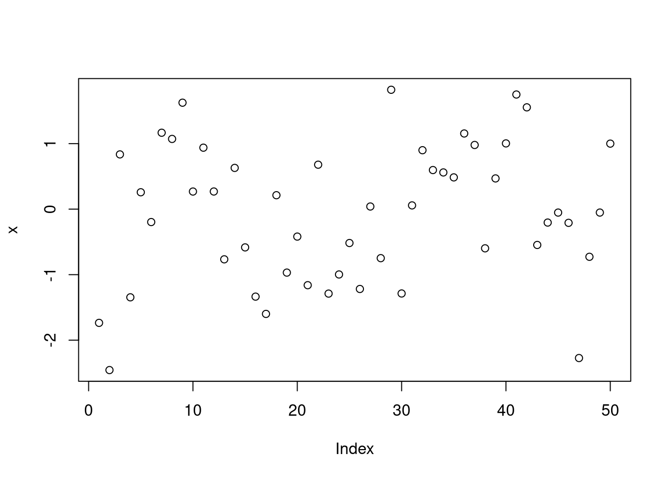
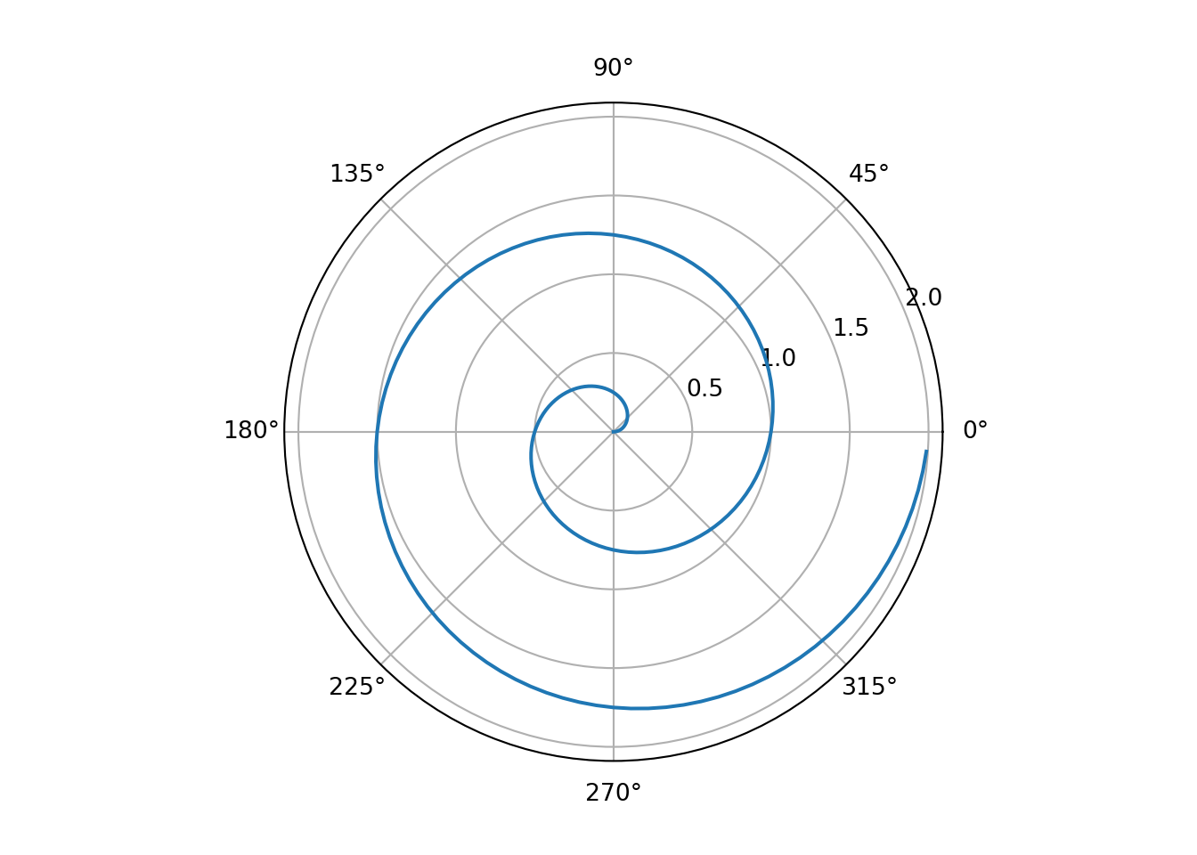
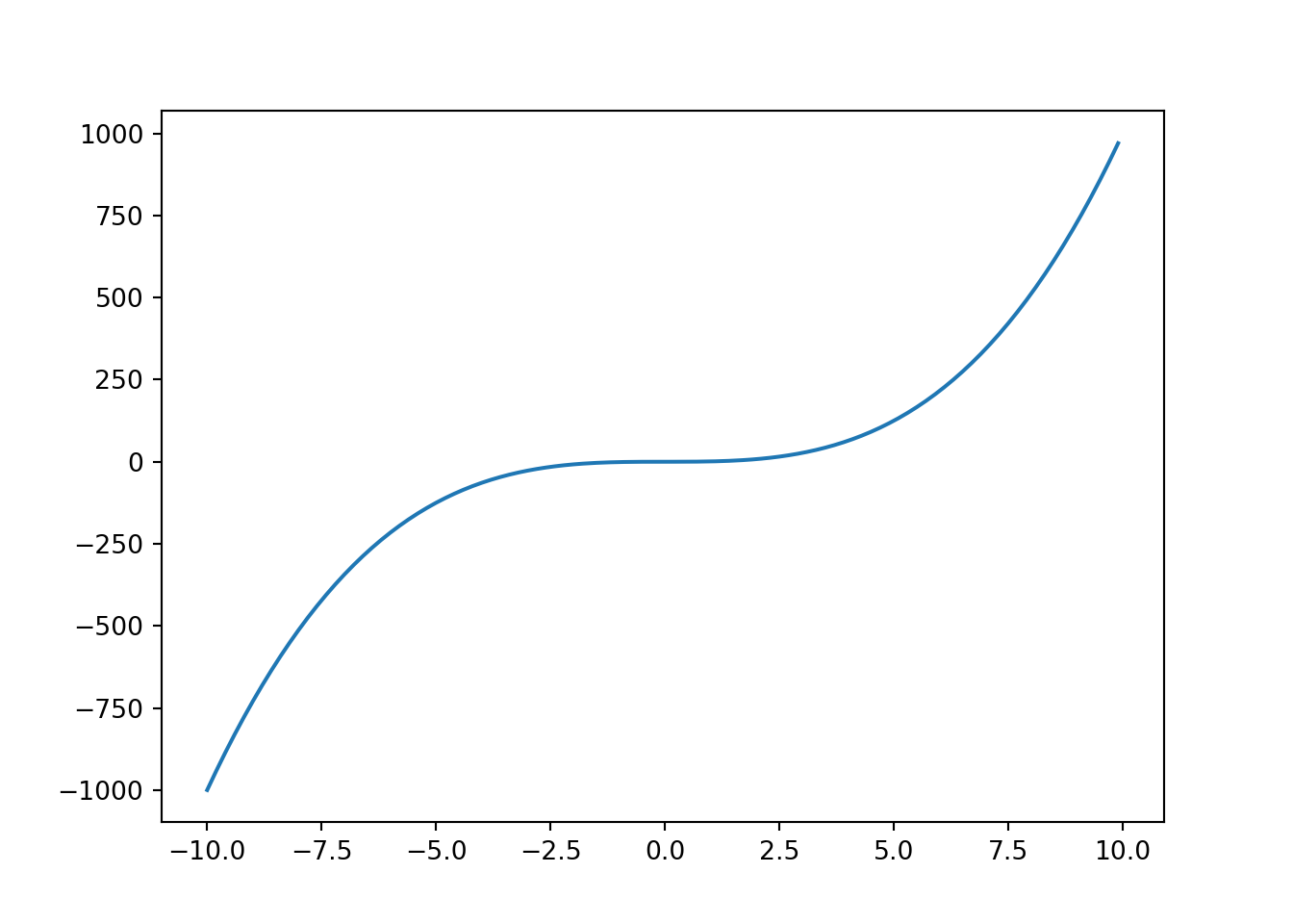
Once the environment is set, you can run Python chunks as usual:
This will demonstrate the R/Python switcher again. Notice this page doesn’t contain the global toggle button in the bottom left as it was disabled at the top of the .qmd, should you wish to disable it.